Lecture 10 Multivariate distributions
Learning objectives
- Define a joint probability density function
- Condition PDFs on other random variables
- Identify independence between two random variables
- Define covariance and correlation
- Examine sums of random variables
- Define the multivariate normal distribution
Supplemental readings
- Chapters 2.5-.7, 3.4-5, 4.2, 4.5, Bertsekas and Tsitsiklis (2008)
- Equivalent reading from Bertsekas and Tsitsiklis lecture notes
10.1 Multivariate distribution
Definition 10.1 (Multivariate distribution) We will say that \(X\) and \(Y\) are jointly continuous if, for all \(x\in\Re\) and \(y\in \Re\), there exists a function \(f(x,y)\) such that \(C \subset \Re^{2}\),
\[\Pr\{(X, Y) \in C \} = \iint_{(x,y)\in C} f(x,y)\, dx\, dy\]
What is \(C \subset R^{2}\)?
\[R^{2} = R \underbrace{\times}_{\text{Cartesian Product}} R\]
This is the 2-d plane (your piece of paper). \(C\) is a subset of the 2-d plane.
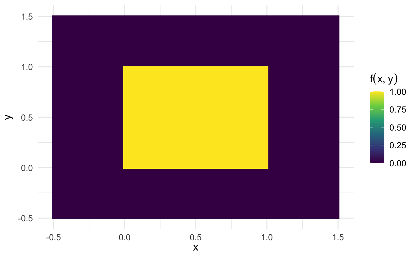
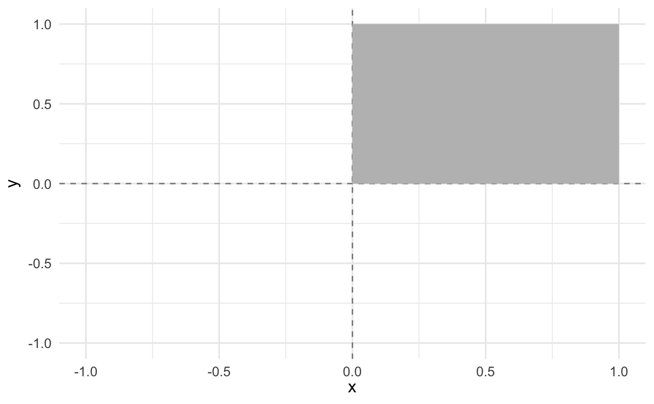
\[C = \{x, y: x \in [0,1] , y\in [0,1] \}\]
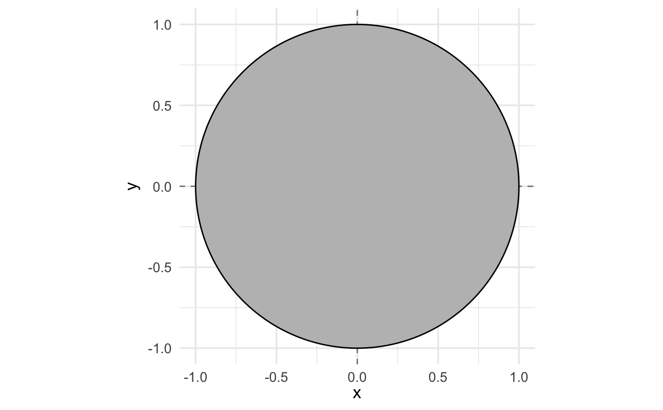
\[C = \{x, y: x^2 + y^2 \leq 1 \}\]
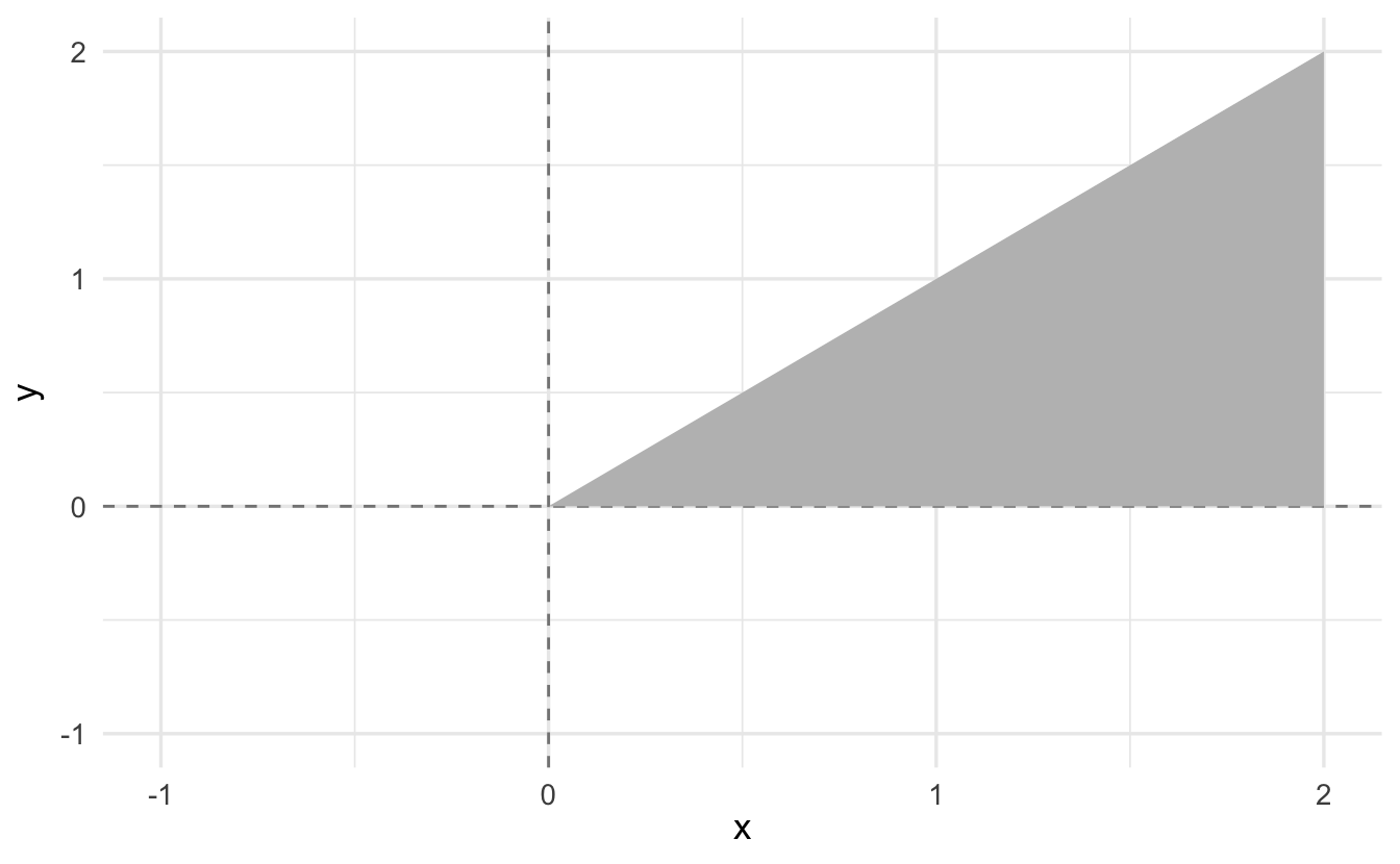
\[C = \{ x, y: x> y, x,y\in(0,2)\}\]
More over, by letting \(C\) be the entire two-dimensional plane, we obtain the normalization property
\[\iint_{(x,y)\in C} f(x,y)\, dx\, dy = 1\]
More generally,
\[ \begin{aligned} C &= \{ x, y: x \in A, y \in B \} \\ \Pr\{(X,Y) \in C \} &= \int_{B} \int_{A} f(x,y) \, dx\, dy \end{aligned} \]
10.2 Examples of joint PDFs
We’re going to focus (initially) on pdfs of two random variables. Consider a function \(f:\Re \times \Re \rightarrow \Re\):
- Input: an \(x\) value and a \(y\) value.
- Output: a number from the real line
- \(f(x,y) = a\)
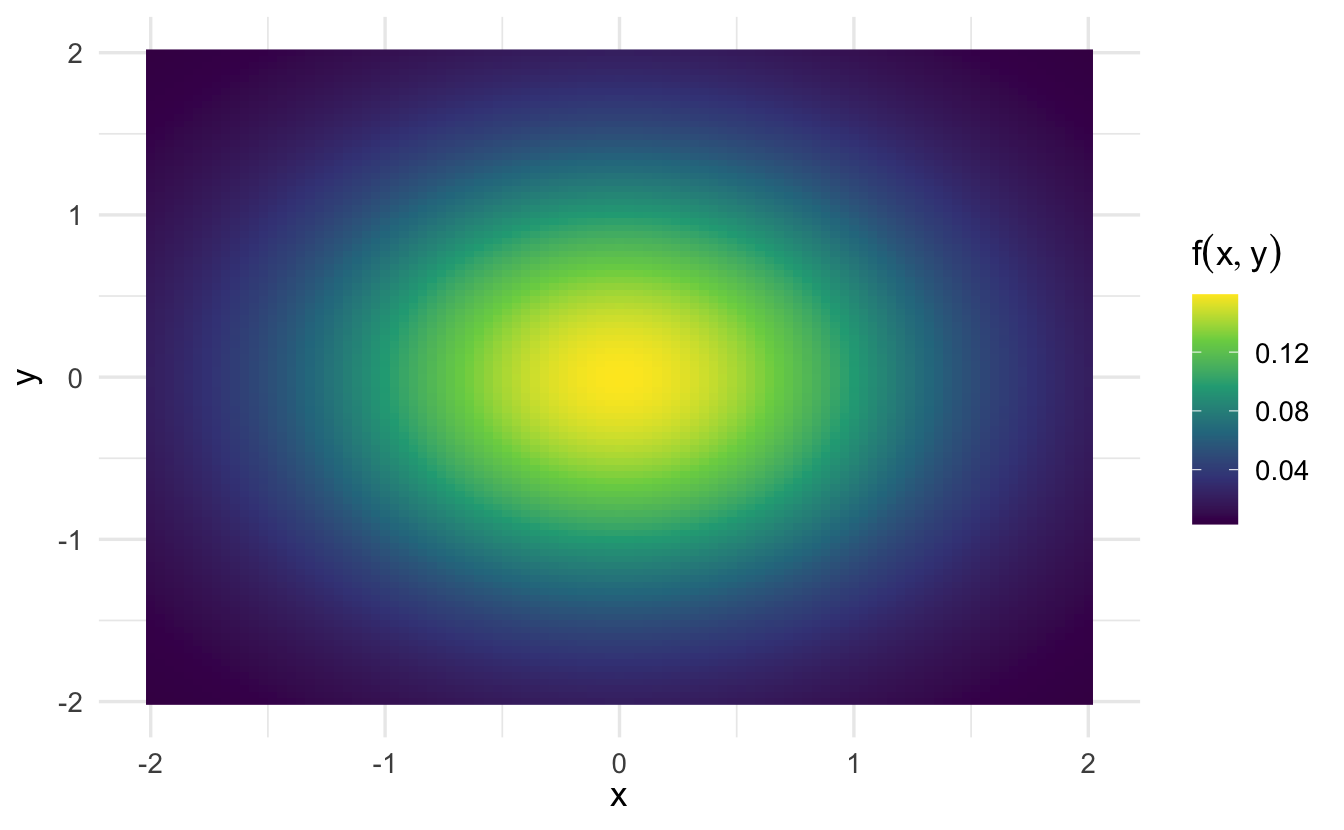
10.2.0.0.1 Multivariate normal distribution
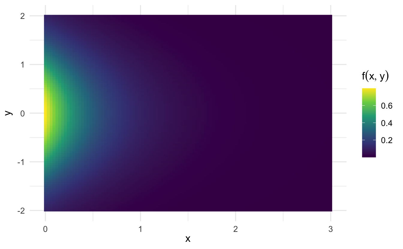
\[ f(x,y) = \frac{1}{2 \pi \sigma_X \sigma_Y \sqrt{1-\rho^2}} \mathrm{e}^{ -\frac{1}{2(1-\rho^2)}\left[ \left(\frac{x-\mu_X}{\sigma_X}\right)^2 - 2\rho\left(\frac{x-\mu_X}{\sigma_X}\right)\left(\frac{y-\mu_Y}{\sigma_Y}\right) + \left(\frac{y-\mu_Y}{\sigma_Y}\right)^2 \right] } \]
where \(\rho\) is the Pearson product-moment correlation coefficient between \(X\) and \(Y\) and where \(\sigma_X>0\) and \(\sigma_Y>0\). In this case,
\[ \boldsymbol\mu = \begin{pmatrix} \mu_X \\ \mu_Y \end{pmatrix}, \quad \boldsymbol\Sigma = \begin{pmatrix} \sigma_X^2 & \rho \sigma_X \sigma_Y \\ \rho \sigma_X \sigma_Y & \sigma_Y^2 \end{pmatrix}. \]
3D plot:
Contour plot:
10.3 Multivariate cumulative density function
Definition 10.2 (Multivariate cumulative density function) For jointly continuous random variables \(X\) and \(Y\) define, \(F(b,a)\) as
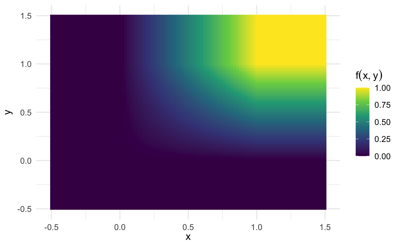
\[F(b,a) = \Pr\{ X \leq b , Y \leq a\} = \int_{-\infty}^{a} \int_{-\infty}^{b} f(x,y) \, dx\, dy\]
10.3.0.0.1 Multivariate normal
\[ f(x,y) = \frac{1}{2 \pi \sigma_X \sigma_Y \sqrt{1-\rho^2}} \mathrm{e}^{ -\frac{1}{2(1-\rho^2)}\left[ \left(\frac{x-\mu_X}{\sigma_X}\right)^2 - 2\rho\left(\frac{x-\mu_X}{\sigma_X}\right)\left(\frac{y-\mu_Y}{\sigma_Y}\right) + \left(\frac{y-\mu_Y}{\sigma_Y}\right)^2 \right] } \]
where \(\rho\) is the Pearson product-moment correlation coefficient between \(X\) and \(Y\) and where \(\sigma_X>0\) and \(\sigma_Y>0\). In this case,
\[ \boldsymbol\mu = \begin{pmatrix} \mu_X \\ \mu_Y \end{pmatrix}, \quad \boldsymbol\Sigma = \begin{pmatrix} \sigma_X^2 & \rho \sigma_X \sigma_Y \\ \rho \sigma_X \sigma_Y & \sigma_Y^2 \end{pmatrix}. \]

10.4 Marginalization
Definition 10.3 (Moving from joint distributions to univariate PDFs) Define \(f_{X}(x)\) as the marginal pdf for \(X\),
\[f_{X}(x) = \int_{-\infty}^{\infty} f(x,y) \, dy\]
Similarly, define \(f_{Y}(y)\) as the marginal pdf for \(Y\),
\[f_{Y}(y) = \int_{-\infty}^{\infty} f(x,y)\, dx\]
Definition 10.4 (Conditional probability distribution function) Suppose \(X\) and \(Y\) are continuous random variables with joint pdf \(f(x,y)\). Then define the conditional probability function \(f(x|y)\) as
\[f(x|y) = \frac{f(x, y) }{f_{Y}(y) }\]
10.4.1 Joint vs. conditional PDF
An example using two standard normal variables \(x\) and \(y\):
\[f(x,y) = x \times y\]
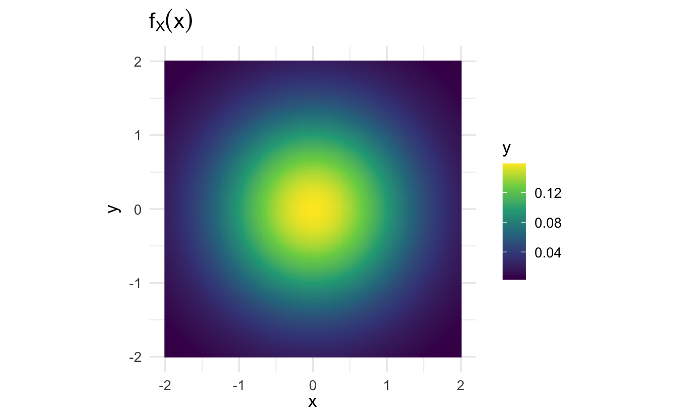
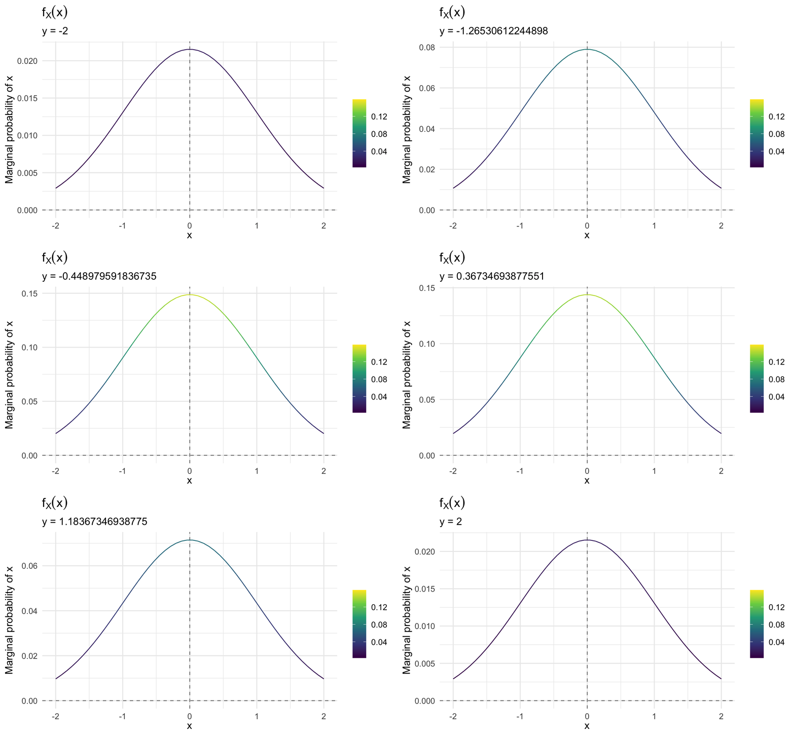
As \(y\) increases, the marginal probability of \(x\) changes.
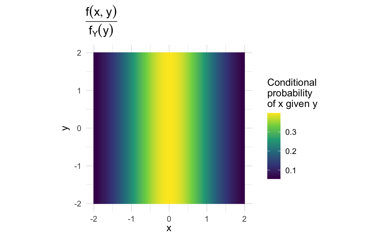
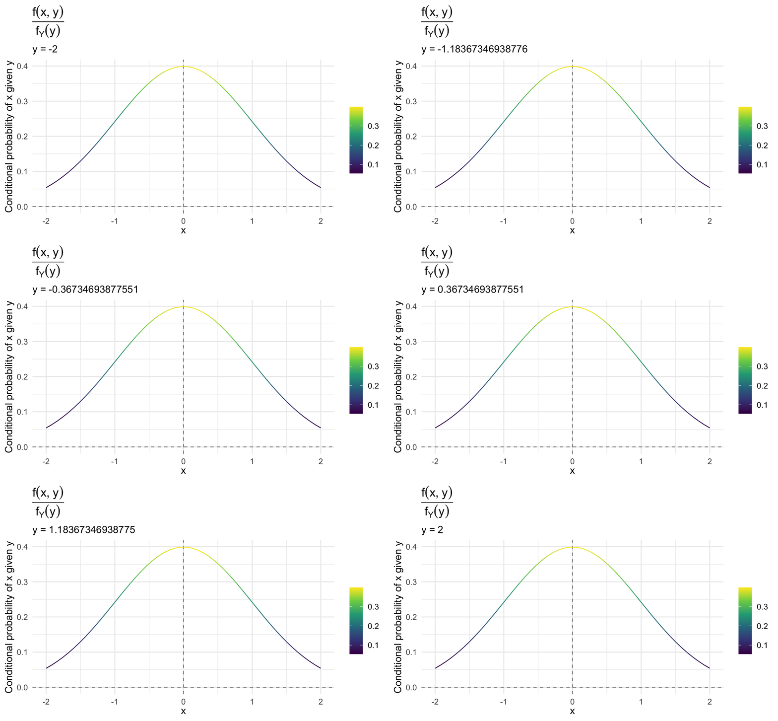
Note that \(f(x | y)\) is the same regardless of the value of \(y\). That is, the conditional probability of \(x\) given \(y\) does not depend on the specific value of \(y\). Why is that?
10.4.2 Why does marginalization work?
Begin with the discrete case.
Consider jointly distributed discrete random variables, \(X\) and \(Y\). We’ll suppose they have a joint PMF,
\[\Pr(X =x, Y = y) = p(x, y)\]
Suppose that the distribution allocates its mass at \(x_{1}, x_{2}, \ldots, x_{M}\) and \(y_{1}, y_{2}, \ldots, y_{N}\). Define the conditional mass function \(\Pr(X= x| Y= y)\) as,
\[ \begin{aligned} \Pr(X=x|Y=y) &\equiv p(x|y) \\ & = \frac{p(x,y)}{p(y)} \end{aligned} \]
Then it follows that:
\[p(x,y) = p(x|y)p(y)\]
Marginalizing over \(y\) to get \(p(x)\) is then,
\[p(x_{j}) = \sum_{i=1}^{N} p(x_{j} |y_{i})p(y_{i} )\]
10.4.2.0.1 Table setup
| \(Y = 0\) | \(Y = 1\) | ||
|---|---|---|---|
| \(X = 0\) | \(p(0,0)\) | \(p(0, 1)\) | \(p_{X}(0)\) |
| \(X = 1\) | \(p(1,0)\) | \(p(1,1)\) | \(p_{X}(1)\) |
| \(p_{Y} (0)\) | \(p_{Y} (1)\) |
10.4.2.0.2 Example probabilities
| \(Y = 0\) | \(Y = 1\) | ||
|---|---|---|---|
| \(X = 0\) | \(0.01\) | \(0.05\) | \(p_{X}(0)\)? |
| \(X = 1\) | \(0.25\) | \(0.69\) | \(p_{X}(1)\)? |
| \(0.26\) | \(0.74\) |
10.4.2.0.3 Marginalize over columns
\[ \begin{aligned} p_{X}(0) & = \Pr(0|y = 0) \Pr(y= 0) + \Pr(0|y=1) \Pr(y=1) \\ & = \frac{0.01}{0.26} \times 0.26 + \frac{0.05}{0.74} \times 0.74 \\ & = 0.06 \end{aligned} \]
\[ \begin{aligned} p_{X}(1) & = \Pr(1|y = 0) \Pr(y= 0) + \Pr(1|y=1) \Pr(y=1) \\ & = \frac{0.25}{0.26} \times 0.26 + \frac{0.69}{0.74} \times 0.74 \\ & = 0.94 \end{aligned} \]
10.4.3 Move to the continuous case
For jointly distributed continuous random variables \(X\) and \(Y\) define,
\[f_{X|Y}(x|y) = \frac{f(x,y)}{f_{Y}(y) }\]
Then, analogously, we can define
\[f_{X}(x) = \int_{-\infty }^{\infty} f_{X|Y}(x|y)f_{Y}(y) \, dy\]
Think of \(f_{X|Y}(x|y)\) as the pdf for \(X\) at a value of \(Y\). We average over those pdfs to get the final pdf for \(X\) (we want densities where there is lots of area of \(Y\) to receive lots of weight, whereas the densities without much area from \(Y\) should receive little weight).
10.4.4 A (simple) example
Suppose \(X\) and \(Y\) are jointly continuous and that
\[ \begin{aligned} f_{XY}(x,y) & = x + \frac{3}{2}y^2 \text{ , if } x \in [0,1], y \in [0,1] \\ & = 0 \text{ , otherwise } \end{aligned} \]
We can show this function is a joint PDF since the area under the multivariate curve is 1.
\[ \begin{aligned} \iint_{-\infty}^{+ \infty} \, dy \, dx &= \iint_0^1 x + \frac{3}{2}y^2 \, dy \, dx \\ &= \int_0^1 \left[ \frac{1}{2} x^2 + \frac{3}{2}y^2x \right]_0^1 \, dy \\ &= \int_0^1 \frac{1}{2} + \frac{3}{2}y^2 \, dy \\ &= \frac{1}{2} \int_0^1 1 \, dy + \frac{3}{2} \int_0^1 y^2 \, dy \\ &= \left[ \frac{y}{2} \right]_0^1 + \left[\frac{y^3}{2} \right]_0^1 \\ &= \frac{1}{2} + \frac{1}{2} \\ &= 1 \end{aligned} \]
We want \(f_{X}(x)\). Assume we have
\[f_{Y}(y) = y\]
Then
\[f_{X|Y}(x|y) = \frac{x + \frac{3}{2}y^2}{y}\]
\[ \begin{aligned} f_X(x) &= \int_{0}^{1} f(x|y)f(y)\, dy \\ &= \int_0^1 \frac{x + \frac{3}{2}y^2}{y} (y) \, dy \\ &= \int_0^1 x + \frac{3}{2}y^2\, dy \\ &= x \int_0^1 1 \, dy + \frac{3}{2} \int_0^1 y^2 \, dy \\ &= x \left[y \right]_0^1 + \frac{3}{2} \left[\frac{y^3}{3} \right]_0^1 \\ &= \left[xy \right]_0^1 + \left[\frac{y^3}{2} \right]_0^1 \\ &= x + \frac{1}{2} \end{aligned} \]
10.4.5 More complex example
Suppose \(X\) and \(Y\) are jointly distributed with PDF
\[f(x,y) = 2 \exp(-x) \exp(-2y), \forall \, x>0, y>0)\]
10.4.5.1 Verify this is a PDF
\[ \begin{aligned} \int_{0}^{\infty} \int_{0}^{\infty} f(x, y) & = 2\int_{0}^{\infty} \int_{0}^{\infty} \exp(-x) \exp(-2y) \, dx\, dy \\ & = 2 \int_{0}^{\infty}\exp(-2y) \, dy \int_{0}^{\infty} \exp(-x) \, dx \\ & = 2 (-\frac{1}{2} \exp(-2y)|_{0}^{\infty} ) ( - \exp(-x)|_{0}^{\infty} ) \\ & = 2\left[ (-\frac{1}{2}(\lim_{y\rightarrow\infty} \exp(-2y) - 1))(- (\lim_{x\rightarrow \infty} \exp(-x) - 1) ) \right] \\ & = 2 \left[ -\frac{1}{2} (-1) \times -1 (-1) \right] \\ & = 1 \end{aligned} \]
10.4.5.2 Calculate CDF
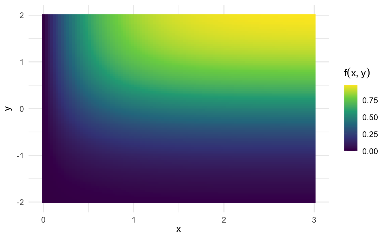
\[ \begin{aligned} F(x,y) \equiv \Pr\{X \leq b, Y \leq a\} & = 2 \int_{0}^{a} \int_{0}^{b} \exp(-x) \exp(-2y) \, dx\, dy \\ & = 2 (\int_{0}^{a} \exp(-2y) \, dy) (\int_{0}^{b} \exp(-x) \, dx) \\ & = 2 \left[-\frac{1}{2} (\exp(-2a) -1 )\right]\left[ - (\exp(-b) - 1) \right] \\ & = \left[1 - \exp(-2a) \right] \left[ 1- \exp(-b) \right] \end{aligned} \]
10.4.5.3 Calculate \(f_{X}(x)\) and \(f_{Y}(y)\)
\[ \begin{aligned} f_{X}(x) & = \int_{0}^{\infty} 2\exp(-x) \exp(-2y) \, dy \\ & = 2 \exp(-x) \int_{0}^{\infty} \exp(-2y) \, dy \\ & = 2 \exp(-x) \left[ -\frac{1}{2}(0 - 1) \right] \\ & = \exp(-x) \end{aligned} \]
\[ \begin{aligned} f_{Y}(y) & = \int_{0}^{\infty} 2 \exp(-x) \exp(-2y) \, dx \\ & = 2 \exp(-2y) \int_{0}^{\infty} \exp(-x) \, dx \\ & = 2 \exp(-2y) \left[-(0 -1) \right] \\ & = 2 \exp(-2y) \end{aligned} \]
10.5 Conditional distribution
Definition 10.5 Two random variables \(X\) and \(Y\) are independent if for any two sets of real numbers \(A\) and \(B\),
\[\Pr\{ X \in A , Y \in B \} = \Pr\{X \in A\} \Pr\{Y \in B\}\]
Equivalently we will say \(X\) and \(Y\) are independent if,
\[f(x,y) = f_{X}(x) f_{Y}(y)\]
If \(X\) and \(Y\) are not independent, we will say they are dependent.
If \(X\) and \(Y\) are independent, then
\[ \begin{aligned} f_{X|Y} (x|y) & = \frac{f(x,y)}{f_{Y}(y)} \\ & = \frac{f_{X}(x)f_{Y}(y)}{f_{Y}(y) } \\ & = f_{X}(x) \end{aligned} \]
10.5.1 A (simple) example of dependence
Suppose \(X\) and \(Y\) are jointly continuous and that
\[ \begin{eqnarray} f(x,y) & = & x + y \text{ , if } x \in [0,1], y \in [0,1] \\ & = & 0 \text{ , otherwise } \end{eqnarray} \]
\[ \begin{eqnarray} f_{X}(x) & = & \int_{0}^{1} \left(x + y \right) \, dy \\ & = & xy + \frac{y^2}{2} |^{1}_{0} \\ & = & x + \frac{1}{2} \\ f_{Y}(y) & = & \frac{1}{2} + y \end{eqnarray} \]
\[ \begin{eqnarray} f(x, y) &= & x + y \\ f_{X}(x) f_{Y}(y) & = & (\frac{1}{2} + x) (\frac{1}{2} + y) \\ & = & \frac{1}{4} + \frac{x + y}{2} + xy \end{eqnarray} \]
Intuition: at different levels of \(X\) the distribution on \(Y\) behaves differently. \(X\) provides information about \(Y\).
10.6 Expectation
Definition 10.6 For jointly continuous random variables \(X\) and \(Y\) define,
\[ \begin{eqnarray} \E[X] & = & \int_{-\infty}^{\infty} \int_{-\infty}^{\infty} x f(x,y) \, dx\, dy \\ \E[Y] & = & \int_{-\infty}^{\infty} \int_{-\infty}^{\infty} y f(x,y) \, dx\, dy \\ \E[XY] & = & \int_{-\infty}^{\infty} \int_{-\infty}^{\infty} x y f(x,y) \, dx\, dy \end{eqnarray} \]
Proposition 10.1 Suppose \(g:\Re^{2} \rightarrow \Re\). Then
\[\E[g(X, Y)] = \int_{-\infty}^{\infty} \int_{-\infty}^{\infty} g(x, y) f(x,y) \, dx\, dy\]
10.7 Covariance and correlation
Definition 10.7 (Covariance) For jointly continous random variables \(X\) and \(Y\) define, the covariance of \(X\) and \(Y\) as,
\[ \begin{align} \Cov(X, Y) &= \E\left[\left(X - \E\left[X\right]\right) \left(Y - \E\left[Y\right]\right)\right] \\ &= \E\left[X Y - X \E\left[Y\right] - \E\left[X\right] Y + \E\left[X\right] \E\left[Y\right]\right] \\ &= \E\left[X Y\right] - \E\left[X\right] \E\left[Y\right] - \E\left[X\right] \E\left[Y\right] + \E\left[X\right] \E\left[Y\right] \\ &= \E\left[X Y\right] - \E\left[X\right] \E\left[Y\right] \end{align} \]
Definition 10.8 (Correlation) Define the correlation of \(X\) and \(Y\) as,
\[\Cor(X,Y) = \frac{\Cov(X,Y) }{\sqrt{\Var(X) \Var(Y) } }\]
10.7.1 Some observations
10.7.1.1 Variance is the covariance of a random variable with itself
\[ \begin{eqnarray} \Cov(X,X) & = & \E[X X] - \E[X]\E[X] \\ & = & \E[X^2] - \E[X]^2 \end{eqnarray} \]
10.7.1.2 Correlation measures the linear relationship between two random variables
Suppose \(X = Y\):
\[ \begin{eqnarray} \Cor(X,Y) & = & \frac{\Cov(X,Y)}{\sqrt{\Var(X)\Var(Y)} } \\ & = & \frac{\Var(X)}{\Var(X)} \\ & = & 1 \end{eqnarray} \]
Suppose \(X = -Y\):
\[ \begin{eqnarray} \Cor(X,Y) & = & \frac{\Cov(X,Y)}{\sqrt{\Var(X)\Var(Y)} } \\ & = & \frac{- \Var(X)}{\Var(X)} \\ & = & -1 \end{eqnarray} \]
10.8 Sums of random variables
Suppose we have a sequence of random variables \(X_{i}\) , \(i = 1, 2, \ldots, N\) and that they have joint pdf
\[f(\boldsymbol{x}) = f(x_{1}, x_{2}, \ldots, x_{n})\]
- \(\E[\sum_{i=1}^{N}X_{i} ] = \sum_{i=1}^{N} \E[X_{i}]\)
- \(\Var(\sum_{i=1}^{N} X_{i} ) = \sum_{i=1}^{N} \Var(X_{i} ) + 2 \sum_{i<j} \Cov(X_{i}, X_{j})\)
Proposition 10.2 Suppose we have a sequence of random variables \(X_{i}\) , \(i = 1, 2, \ldots, N\).
Suppose that they have joint pdf,
\[f(\boldsymbol{x}) = f(x_{1}, x_{2}, \ldots, x_{n})\]
Then
\[\E[\sum_{i=1}^{N} X_{i} ] = \sum_{i=1}^{N} \E[X_{i} ]\]
Proof. \[ \begin{eqnarray} \E[\sum_{i=1}^{N} X_{i} ] & = & \E[X_{1} + X_{2} + \ldots + X_{N}] \\ & = & \int_{-\infty}^{\infty} \cdot \cdot \cdot \iint_{-\infty}^{\infty} (x_{1} + x_{2} + \ldots + x_{N}) f(x_{1}, x_{2}, \ldots, x_{N}) \, dx_{1}\, dx_{2}\ldots \, dx_{N} \\ & = & \int_{-\infty}^{\infty}x_{1} f_{X_{1}}(x_{1}) \, dx_{1} + \int_{-\infty}^{\infty}x_{2} f_{X_{2}}(x_{2}) \, dx_{2} + \ldots + \int_{-\infty}^{\infty}x_{N} f_{X_{N}}(x_{N}) \, dx_{N} \\ & = & \E[X_{1} ] + \E[X_{2}] + \ldots + \E[X_{N}] \end{eqnarray} \]
Proposition 10.3 Suppose \(X_{i}\) is a sequence of random variables. Then
\[ \begin{eqnarray} \Var(\sum_{i=1}^{N} X_{i} ) & = & \sum_{i=1}^{N} \Var(X_{i} ) + 2 \sum_{i<j} \Cov(X_{i}, X_{j} ) \end{eqnarray} \]
Proof. Consider two random variables, \(X_{1}\) and \(X_{2}\). Then,
\[ \begin{eqnarray} \Var(X_{1} + X_{2} ) & = & \E[(X_{1} + X_{2})^2] - \left(\E[X_{1}] + \E[X_{2}] \right)^2 \\ & = & \E[X_{1}^2] + 2 \E[X_{1}X_{2}] + \E[X_{2}^2] \\ && - (\E[X_{1}])^2 - 2 \E[X_{1}] \E[X_{2}] - 2 \E[X_{2}]^2 \\ & = & \underbrace{\E[X_{1}^2] - (\E[X_{1}])^2}_{\Var(X_{1}) } + \underbrace{\E[X_{2}^2] - \E[X_{2}]^{2}}_{\Var(X_{2})} \\ && + 2 \underbrace{(\E[X_{1} X_{2} ] - \E[X_{1}] \E[X_{2} ] )}_{\Cov(X_{1}, X_{2} ) } \\ & = & \Var(X_{1} ) + \Var(X_{2} ) + 2 \Cov(X_{1}, X_{2}) \end{eqnarray} \]
10.9 Multivariate normal distribution
Definition 10.9 (Multivariate normal distribution) Suppose \(\boldsymbol{X} = (X_{1}, X_{2}, \ldots, X_{N})\) is a vector of random variables. If \(\boldsymbol{X}\) has pdf
\[f(\boldsymbol{x}) = (2 \pi)^{-N/2} \text{det}\left(\boldsymbol{\Sigma}\right)^{-1/2} \exp\left(-\frac{1}{2}(\boldsymbol{x} - \boldsymbol{\mu})^{'}\boldsymbol{\Sigma}^{-1} (\boldsymbol{x} - \boldsymbol{\mu} ) \right)\]
Then we will say \(\boldsymbol{X}\) is a Multivariate Normal Distribution,
\[\boldsymbol{X} \sim \text{Multivariate Normal} (\boldsymbol{\mu}, \boldsymbol{\Sigma})\]
This is regularly used for likelihood, Bayesian, and other parametric inferences.
10.9.1 Bivariate example
Consider the (bivariate) special case where \(\boldsymbol{\mu} = (0, 0)\) and
\[ \boldsymbol{\Sigma} = \begin{pmatrix} 1 & 0 \\ 0 & 1 \\ \end{pmatrix} \]
Then
\[ \begin{eqnarray} f(x_{1}, x_{2} ) & = & (2\pi)^{-2/2} 1^{-1/2} \exp\left(-\frac{1}{2}\left( (\boldsymbol{x} - \boldsymbol{0} ) ^{'} \begin{pmatrix} 1 & 0 \\ 0 & 1 \\ \end{pmatrix} (\boldsymbol{x} - \boldsymbol{0} ) \right) \right) \\ & = & \frac{1}{2\pi} \exp\left(-\frac{1}{2} (x_{1}^{2} + x_{2} ^ 2 ) \right) \\ & = & \frac{1}{\sqrt{2\pi}} \exp\left(-\frac{x_{1}^{2}}{2} \right) \frac{1}{\sqrt{2\pi}} \exp\left(-\frac{x_{2}^{2}}{2} \right) \end{eqnarray} \]
\(\leadsto\) product of univariate standard normally distributed random variables
Definition 10.10 (Standard multivariate normal distribution) Suppose \(\boldsymbol{Z} = (Z_{1}, Z_{2}, \ldots, Z_{N})\) is
\[\boldsymbol{Z} \sim \text{Multivariate Normal}(\boldsymbol{0}, \boldsymbol{I}_{N} )\]
Then we will call \(\boldsymbol{Z}\) the standard multivariate normal.
10.9.2 Properties of the multivariate normal distribution
Suppose \(\boldsymbol{X} = (X_{1}, X_{2}, \ldots, X_{N} )\)
\[ \begin{eqnarray} \E[\boldsymbol{X} ] & = & \boldsymbol{\mu} \\ \Cov(\boldsymbol{X} ) & = & \boldsymbol{\Sigma} \end{eqnarray} \]
So that,
\[ \begin{eqnarray} \boldsymbol{\Sigma} & = & \begin{pmatrix} \Var(X_{1}) & \Cov(X_{1}, X_{2}) & \ldots & \Cov(X_{1}, X_{N}) \\ \Cov(X_{2}, X_{1}) & \Var(X_{2}) & \ldots & \Cov(X_{2}, X_{N} ) \\ \vdots & \vdots & \ddots & \vdots \\ \Cov(X_{N}, X_{1} ) & \Cov(X_{N}, X_{2} ) & \ldots & \Var(X_{N} ) \\ \end{pmatrix} \end{eqnarray} \]
10.9.3 Independence and multivariate normal
Proposition 10.4 Suppose \(X\) and \(Y\) are independent. Then
\[\Cov(X, Y) = 0\]
Proof. Suppose \(X\) and \(Y\) are independent.
\[\Cov(X, Y) = \E[XY] - \E[X]\E[Y]\]
Calculating \(\E[XY]\)
\[ \begin{eqnarray} \E[XY] & = & \int_{-\infty}^{\infty} \int_{-\infty}^{\infty} x y f(x,y)\, dx\, dy \\ & =& \int_{-\infty}^{\infty} \int_{-\infty}^{\infty} x y f_{X}(x) f_{Y}(y)\, dx\, dy \\ & = & \int_{-\infty}^{\infty} x f_{X}(x) \, dx \int_{-\infty}^{\infty} y f_{Y}(y) \, dy \\ & = & \E[X] \E[Y] \end{eqnarray} \]
Then \(\Cov(X,Y) = 0\).
Zero covariance does not generally imply independence!
Example 10.1 (Dependent variables with zero covariance) Suppose \(X \in \{-1, 1\}\) with \(\Pr(X = 1) = \Pr(X = -1) = 1/2\).
Suppose \(Y \in \{-1, 0,1\}\) with \(Y = 0\) if \(X = -1\) and \(\Pr(Y = 1) = \Pr(Y= -1)\) if \(X = 1\).
\[ \begin{eqnarray} \E[XY] & = & \sum_{i \in \{-1, 1\} } \sum_{j \in \{-1, 0, 1\}} i j \Pr(X = i, Y = j) \\ & = & -1 \times 0 \times \Pr(X = -1, Y = 0) + 1 \times 1 \times \Pr(X = 1, Y = 1) \\ && - 1 \times 1 \times \Pr(X = 1, Y = -1) \\ &= & 0 + \Pr(X = 1, Y = 1) - \Pr(X = 1, Y = -1 ) \\ & = & 0.25 - 0.25 = 0 \\ \E[X] & = & 0 \\ \E[Y] & = & 0 \end{eqnarray} \]
Proposition 10.5 Suppose \(\boldsymbol{X} \sim \text{Multivariate Normal}(\boldsymbol{\mu}, \boldsymbol{\Sigma})\), where \(\boldsymbol{X}= (X_{1}, X_{2}, \ldots, X_{N})\).
If \(\Cov(X_{i}, X_{j}) = 0\), then \(X_{i}\) and \(X_{j}\) are independent.
